Determining Size and Shape Parameters from Small-Angle Scattering Data using Invertible Neural Networks
- Sofya Laskina, Brian R. Pauw, and Philipp Benner
- Federal Institute for Materials Research and Testing (BAM), Unter den Eichen 87, 12205 Berlin, Germany
- philipp.benner@bam.de, brian.pauw@bam.de
[DRAFT]
Abstract
Scattering techniques, such as small-angle X-ray or neutron scattering, provide information on the fine structure of materials by measuring the intensity of waves scattered via an interference process.
While this interference process can be accurately described in mathematics as a Fourier transform of the probed electron density, not all the information contained therein is recorded in the measurement process. The information loss is of such a magnitude that the retrieval of practically-relevant structural information falls under the class of inverse problems.
For analyzing single datasets, a bespoken model can usually be constructed. For processing larger quantities of data, however, such as collected at well-functioning laboratory instruments or large facilities, an initial clustering and indication of the class and size of scatterers involved would already be a good step forwards. A reliable, universal clustering method does not exist as yet.
We attempt to address this problem using invertible neural networks trained on theoretical scatterers with their analytical SAS intensities. Somewhat surprisingly, our method is able to reliably identify size and shape parameters. This shows that invertible neural networks may have large potential to help interpret small-angle scattering measurements. Ideally, we hope that this work is a first step towards a fully automated SAS data processing workflow.
Software: https://github.com/pbenner/ixs
Introduction
Since its inception in the very beginning of the 20th century, small-angle scattering methods have provided some insight into the fine structure of materials, elucidating structures with dimensions including (and occasionally exceeding) 1-100 nm. While the experiments are straightforward, the data correction and analysis is not. With increasing amounts of data flowing from the instruments, an urgent need arises for the development of automatable analysis solutions.
Analysis of small-angle scattering patterns has evolved in great strides over the last century. Initially, only generic, unreliable information could be deduced from linearization of unreliably recorded scattering intensity (a notable example where both the data as well as the analysis method was unreliable). With the increasing availability of computing power, least-squares minimization methods could become mainstream, although they still rely on models that can be parameterized using only a handful of free parameters. More advanced analyses nowadays no longer require the distribution form to be defined, but return a parameter (typically size-) distribution when a scatterer shape is defined. Whether or not both size distribution parameters as well as shape classes can be determined remains an open question. Even an initial guess, however, would be helpful in tackling the vast amounts of data currently collected in laboratories and large facilities worldwide.
Invertible neural networks (INNs) [1; 2] are a promising alternative to existing methods for estimating material characterstics from SAS measurements. These methods specifically address surjective problems, where the measurement data is not sufficient for recovering all information about a sample. As opposed to traditional methods, where this gap is filled with prior assumptions, INNs learn this information entirely from training data. This makes INNs ideal for applications where prior information is difficult to be expressed in mathematical terms, however, at the cost of having to collect a sufficiently large set of training data, which is representative for the experimental setup at hand. In addition, INNs are probabilistic models and their invaluable strength is that they allow to recover a full distribution of feasible solutions. Other machine learning models have been applied to SAS data [3; 4; 5], but they do not address the surjective nature of the inverse problem.
In this study, we consider small-angle scattering data of isotropically scattering, size-disperse systems. We create a large data set of simulated theoretical scatterers with varying shapes and sized and their corresponding intensity curves. This data is used to train our INN (i.e. estimate the parameters of the model) and we show that our model is capable of recovering size and shape parameters of the theoretical scatterers with high precision. In addition, we provide a software package of our model that can be easily applied to other data sets. This allows researchers to train models that are capable of predicting size and shape parameters for their domain of interest, given that a sufficiently large data set of simulated or experimental SAS measurements with known parameters is available.
Results
Synthetic data
The synthetic data is generated by drawing size and shape parameters at random. For each sampled set of parameters, the one-dimensional scattering curve is computed using an analytical solution implemented in SasView. We set the size of the simulation box in real space to $l = 100~nm$. The one-dimensional intensity is computed for $n$ scattering angles $q = \log(0.03), \dots, \log(3)$ (evenly spaced on log-scale). In all simulations, the scattering length density (SLD) is set to one for the scatterer and zero for the solvent. We decided to restrict the data set to three shapes, namely, spheres, hardspheres, and cylinders. For each of the shapes, we created 5000 samples.
| cylinder | sphere | hard sphere | |
|---|---|---|---|
| radius | $\mathcal{N}(2, 1)$ | $\mathcal{N}(2, 1)$ | $\mathcal{N}(2, 1)$ |
| radius polydispersity | $\mathcal{N}(0.1, 0.03)$ | $\mathcal{N}(0.1, 0.03)$ | $\mathcal{N}(0.1, 0.03)$ |
| length | $\mathcal{N}(10, 5)$ | — | — |
| length polydispersity | $\mathcal{N}(0.1, 0.03)$ | — | — |
| volume fraction | $\mathcal{N}(0.2, 0.01)$ | $\mathcal{N}(0.2, 0.01)$ | $\mathcal{N}(0.2, 0.01)$ |
Table 1: Distributions of parameters for generating synthetic data. The normal distributions $\mathcal{N}(\mu, \sigma)$ are parameterized by their mean $\mu$ and standard deviation $\sigma$.
The parameters for generating the synthetic data are given in Table 1. For all three shapes we have as parameters the radius and the radius polydispersity. Both parameters are assumed to follow a Gaussian distribution. While the distribution of the radius defines the variation between samples, the polydispersity introduces variation of the radius within a sample. The hard sphere and cylinder have additional parameters. For hard spheres we set the effective radius, which represents the interaction radius of a particle, equal to the actual radius. For instance, due to charges the effective radius might be greater than the actual radius of the particle. Many such interactions exist that can adjust the effective radius compared to the real radius. The volume fraction parameter regulates how densely the simulation box is filled. It is drawn with equal probability from a set of 7 values (see Table 1). For the cylinders, the angular parameters are not specified, because they are not captured by one-dimensional scattering curves. Finally, we applied some noise to the simulations. The simulated intensity is multiplied at each scattering angle $q$ by a random value drawn from a normal distribution with mean $\mu = 1$ and standard deviation $\sigma = 0.1$, which we selected because the resulting scattering intensities closely resemble experimental ones. The mean and 95% quantile of the simulated data is shown in Figure 1.
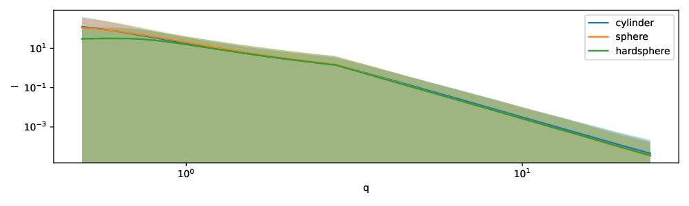
Figure 1: Mean and 95% quantile of synthetic intensity curves stratified by shape
Prediction of size and shape parameters
In our approach, we specifically want to address the surjectivity of the inverse scattering problem. There exist several machine learning models that are designed for inverse problems, the most important, among others, are i-ResNet [2] and conditional RNVP [1]. The i-ResNet approach puts constraints on the Jacobian of the neural network model, thereby allowing the computation of the inverse through simple fixed point iterations. The disadvantage of this approach is on the one hand the computational cost and on the other hand a lack of uncertainty quantification. Conditional RNVPs are more appropriate for SAS data, because they belong to the family of generative models and therefore allow to compute multiple inverse solutions that can be aggregated into a mean prediction and an uncertainty measure such as the standard deviation. A full description of the model and our modifications is provided in Section 4. Our software package relies on the implementation of an existing RNVP model [6].
To evaluate our model on the synthetic SAS data, we randomly divided the data into train (90%) and test (10%) data. On the training data, we estimated model parameters using adaptive momentum estimation (Adam) and a plateau scheduler to automatically reduce the learning rate (see Section 4) when needed. A small fraction (10%) of the training data is set apart as validation set to stop training before the model starts overfitting. Figure 2 shows that the training is converging well and that we observe almost no overfitting on the validation data. The test data is then used to evaluate the accuracy of predictions.
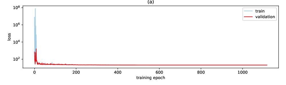
Figure 2: raining and validation loss as a function of epoch during estimation of model parameters
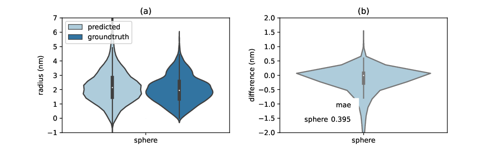
Figure 3: Prediction accuracy of radii. (a) Distributions of predicted and groundtruth radii (b) Distribution of differences between predicted and true radii. The mean absolute error (mae) is shown as table within the figure
Uncertainty quantification
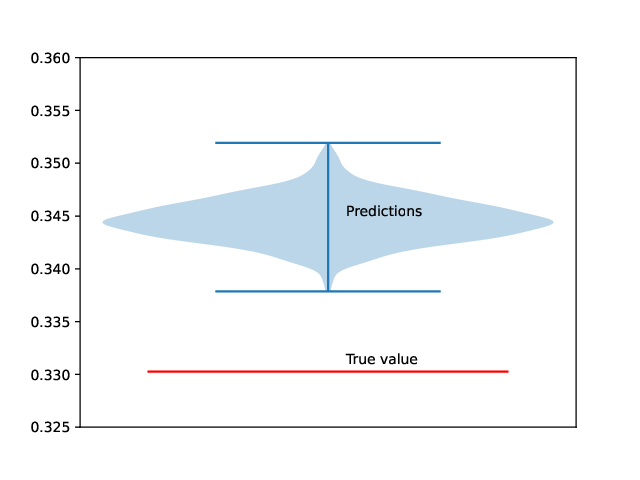
Figure 4: Uncertainty quantification of radius predictions for a cylinder sample. The uncertainty of the model is estimated by repeatedly computing radius predictions for a fixed cylinder scattering curve.
Methods
Machine learning model
An invertible neural network (INN) is a bijective function $f(x) = y$, i.e. there exists an inverse $g = f^{-1}$ such that $x = (g \circ f)(x)$ for all $x$. INN models typically consist of smaller invertible building blocks, also called coupling blocks. Several invertible coupling blocks have been proposed so far. We rely on the RealNVP (RNVP) coupling block [@dinh2016] as defined by \(\begin{aligned} y_1 &= x_1 \odot \exp\left[ s_2(x_2)\right] + t_2(x_2)\\ y_2 &= x_2 \odot \exp\left[ s_1(y_1)\right] + t_1(y_1)\end{aligned}\) where $\odot$ is the element-wise multiplication. Input and output are split into two halves \(x = [x_1, x_2]\,,\quad y = [y_1, y_2]\,.\) and the functions $t_1, t_2, s_1, s_2$ can be chosen arbitrarily, but typically consist of dense neural networks. The splitting of the input allows to easily compute the inverse. When building INN models, it is important to shuffle the inputs to increase the expressiveness of the model.
For surjective problems, the output $y$ contains less information than the input $x$ of the INN model. Conditional RNVPs circumvent this problem by using an augmented output $\tilde{y} = [y, z] = f(x)$, where $z$ is a latent representation of the lost information that is learned during model training [1]. The inverse of an output $y$ is computed by first randomly drawing a value $z$ and then computing the inverse $x = g([y, z])$. Multiple solutions $x$ can be computed by repeating this process, which then allows to provide summary statistics, such as mean and variance.
Acknowledgments
This work benefited from the use of the SasView application, originally developed under NSF award DMR-0520547. SasView contains code developed with funding from the European Union’s Horizon 2020 research and innovation programme under the SINE2020 project, grant agreement No 654000.
References
[1] Lynton Ardizzone, Jakob Kruse, Sebastian Wirkert, Daniel Rahner, Eric W Pellegrini, Ralf S Klessen, Lena Maier-Hein, Carsten Rother, and Ullrich Köthe. Analyzing inverse problems with invertible neural networks. arXiv preprint arXiv:1808.04730, 2018.
[2] Jens Behrmann, Will Grathwohl, Ricky TQ Chen, David Duvenaud, and Jörn-Henrik Jacobsen. Invertible residual networks. In International Conference on Machine Learning, pages 573–582. PMLR, 2019.
[3] Piotr Tomaszewski, Shun Yu, Markus Borg, and Jerk Rönnols. Machine learning-assisted analysis of small angle x-ray scattering. In 2021 Swedish Workshop on Data Science (SweDS), pages 1–6. IEEE, 2021.
[4] Christian Scherdel, Eddi Miller, Gudrun Reichenauer, and Jan Schmitt. Advances in the development of sol-gel materials combining small-angle x-ray scattering (saxs) and machine learning (ml). Processes, 9(4):672, 2021. 10
[5] Magnus Röding, Piotr Tomaszewski, Shun Yu, Markus Borg, and Jerk Rönnols. Machine learning-accelerated small-angle x-ray scattering analysis of disordered two-and three-phase materials. Frontiers in Materials, 9:956839, 2022.
[6] Lynton Ardizzone, Till Bungert, Felix Draxler, Ullrich Köthe, Jakob Kruse, Robert Schmier, and Peter Sorrenson. Framework for Easily Invertible Architectures (FrEIA), 2018-2022. URL https://github.com/vislearn/FrEIA.